Objective/Overview
The objective of this project is to use neural network with keras to solve regression problem in Python and R. This project was originally done in Python in Deep Learning with Keras, from Antonio Gulli and Sujit Pal, Keras regression example - predicting benzene levels in the air. Here we redo this project in Python.
This section executes blue part of the project flow shown in the figure below in R.
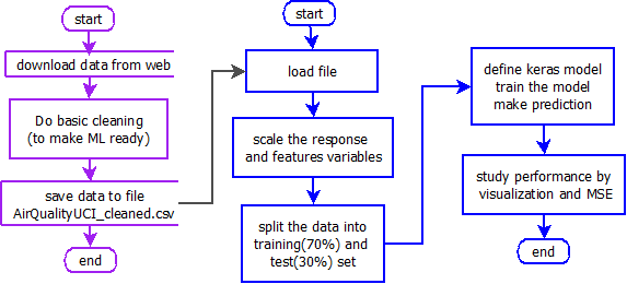
- In previous section (in R shown in purple in figure above), we downloaded the data from web and did some basic cleaning.
- In this section, we do the following
- Load the data which was processed in previous section
- Scale the variables (response and features)
- Split the sample in 70-30 for training and testing
- Define the model with one hidden layer and one output layer. The output layer has no activation function because it is regression problem.
- Run the model and predict for testing
- Meausre the performance with MSE and some visualization
Links
Following are the links for the code and report generated
Relates to purple part of the project (see figure above).
- Report in R
- Code as Rmd file (executed in Rstudio)
Relates to blue part of the project (see figure above).
- Report in R
- Code as Rmd file (executed in Rstudio)
- Report in Python (This page!)
- Code in Python (executed in Jupyter)
Data source:
Courtesy of https://archive.ics.uci.edu/ml/datasets/Air+Quality
Load Libraries
from keras.layers import Input
from keras.layers.core import Dense
from keras.models import Model
from sklearn.preprocessing import StandardScaler
import matplotlib.pyplot as plt
import numpy as np
import os
import pandas as pd
Read and Split the Data
The following reads the clean data processed in previous section.
DATA_DIR = "c:/ds_local/dataset/"
AIRQUALITY_FILE = os.path.join(DATA_DIR, "AirQualityUCI_cleaned.csv")
aqdf = pd.read_csv(AIRQUALITY_FILE, sep=",", decimal=".", header=0)
# remove first and last 2 cols
#del aqdf["Date"]
#del aqdf["Time"]
#del aqdf["Unnamed: 15"]
#del aqdf["Unnamed: 16"]
# fill NaNs in each column with the mean value
#aqdf = aqdf.fillna(aqdf.mean())
df_data = aqdf.as_matrix()
type(df_data)
scale the variable as, $ z= {{x-\mu}\over{\sigma}} $
scaler = StandardScaler()
trn = scaler.fit_transform(df_data)
# store these off for predictions with unseen data
Xmeans = scaler.mean_
Xstds = scaler.scale_
y_trn = trn[:, 3]
x_trn = np.delete(trn, 3, axis=1)
# split the train and test size as 70:30
train_size = int(0.7 * trn.shape[0])
x_trn_tr, x_trn_te, y_trn_tr, y_trn_te = x_trn[0:train_size], x_trn[train_size:],y_trn[0:train_size], y_trn[train_size:]
Defining the model
- Layer 1: Input layer = No of features = 12
- Layer 2: Hidden layer = 8 (data compression like PCA but non-linear)
- Layer 3: output layer = 1. No activation as response is regression.
## This code works, but written smartly, but I prefer dumb code which is in next cell block
#readings = Input(shape=(12,))
#x = Dense(8, activation="relu", kernel_initializer="glorot_uniform")(readings)
#benzene = Dense(1, kernel_initializer="glorot_uniform")(x)
#model = Model(inputs=[readings], outputs=[benzene])
#model.compile(loss="mse", optimizer="adam")
from keras.models import Sequential
from keras.layers.core import Dense, Activation
model = Sequential()
model.add(Dense(8,input_shape=(12,), kernel_initializer="glorot_uniform"))

#, output_dim=8, kernel_initializer="glorot_uniform"))
model.add(Activation('relu'))
model.add(Dense(units=1, kernel_initializer="glorot_uniform")) # output_dim=1
model.compile(loss="mse", optimizer="adam")
NUM_EPOCHS = 20
BATCH_SIZE = 10
history = model.fit(x_trn_tr, y_trn_tr, batch_size=BATCH_SIZE, epochs=NUM_EPOCHS,
validation_split=0.2)
y_prd = model.predict(x_trn_te).flatten()
y_trn_te_unscaled = (y_trn_te * Xstds[3]) + Xmeans[3]
y_prd_unscaled = (y_prd * Xstds[3]) + Xmeans[3]

for i in range(10):
    y_true_i= (y_trn_te[i] * Xstds[3]) + Xmeans[3]
    y_prd_i = (y_prd[i] * Xstds[3]) + Xmeans[3]
    print("Benzene Conc. expected: {:.3f}, predicted: {:.3f}".format(y_true_i, y_prd_i))
plt.plot(np.arange(y_trn_te.shape[0]), (y_trn_te * Xstds[3]) / Xmeans[3],color="b", label="actual")
plt.plot(np.arange(y_prd.shape[0]), (y_prd * Xstds[3]) / Xmeans[3], color="r", alpha=0.5, label="predicted")
plt.xlabel("time")
plt.ylabel("C6H6 concentrations")
plt.legend(loc="best")
plt.show()

import math
math.sqrt(sum((y_trn_te_unscaled-y_prd_unscaled)**2))/len(y_trn_te_unscaled)
#(y_trn_te_unscaled-y_prd_unscaled)